Links:

COMPARISON OF PERFORMANCE AND COST

OF THREE SOLAR PHOTOVOLTAIC SYSTEMS

The purpose of this section is to compare the performance of several solar photovoltaic (PV) systems made by different manufacturers under actual operating conditions for residential applications.  Another objective is to see how accurately the performance of these systems is predicted by a publically available software package developed by the National Renewable Energy Laboratory (NREL) called “PVWatts 40 km Grid” (or Version 2).  This software computes the estimated AC power with corrections for the PV module temperature's impact on PV efficiency, reflection losses, and inverter efficiency as a function of load, in addition to the derate factors.  The derate factors are discussed in more detail below.  This software package is the most widely used computer model to size solar PV system to meet a specified electrical load, and it is important that it be reasonably accurate.   

These PV systems are all located within a few miles of each other in a sunny, high mountain valley in or near Salida, Colorado (south-central Colorado, zip code 81201).  All systems have been purchased and installed within the last two years.  The annual average solar insolation on a flat plate collector tilted up from horizontal at an angle equal to the latitude is about 5.78 kW/m2/day, according to the National Renewable Energy Laboratory PV Watts Viewer (http://mapserve3.nrel.gov/PVWatts_Viewer/index.html).  This may be compared with other locations in the U.S. as shown for the same units (kW/m2/day) in Figure 1, which is also from NREL (http://www.nrel.gov/gis/images/map_pv_national_lo-res.jpg), and again this is for a collector tilted up at an angle equal to the latitude.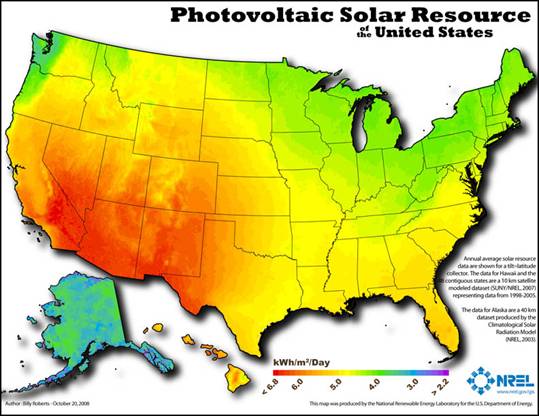    

Figure 1.  Average Annual Solar Insolation on Flat Plate Tilted up at Angle Equal to Latitude.

The three solar systems currently being monitored include those shown in Table 1 below.  These are all standard production systems, and all were professionally installed.  The first two systems, Sun Power and Sharp, were installed in 2010, and the third one, REC, in 2011.  Notice the large variation in PV module efficiency, with the first one significantly higher than the other two.  The cost per installed Watt before subsidies has dropped from about $5.82 in 2010 to about $4.89 in 2011, with further decreases in late 2011.  The subsidized cost varies depending on the utility supplier and the rebate program in place at the time of purchase.  The subsidized cost is only 30% to 50% of the unsubsidized cost for these units, so the subsidies are important in figuring payoff periods for solar PV. 

Table 1.  Solar PV System Characteristics.

Since the three systems all have different ratings, it would be unreasonable to compare their total energy outputs directly.  Rather, since the output power and energy scale directly with the power rating at STC (standard test condition), comparisons of performance are made by normalizing the output energy by the rated power.  This provides results in energy/power, or kWh/kW. 

From Table 1, it may be seen that the PV panels for systems #1 and #2 are at the same orientation, being tilted up from horizontal at 26.6˚ (for a 6:12 pitch roof) compared to a latitude of about 36.5˚, and aimed 22˚ east of due south.  As a first guess, panels should be tilted up from horizontal at an angle approximately equal to the latitude, and oriented due south.  The panels for system #3 are oriented further from the ideal orientation, being tilted up from horizontal by 18.4˚ (for a 4:12 pitch roof), and aimed at 41˚ east of south. 

The effect of aligning the panels in a direction other than the optimum angle is not as strong as might be anticipated, as shown in the figures below.  In the first two figures below, the effect of changing the tilt angle from horizontal (0˚) to vertical (90˚) at the optimum azimuth angle of 169˚ (11˚ east of due south) is shown, and in the next two figures, the effect of changing the azimuth angle from due east (90˚) to due west (270˚) with the tilt fixed at the optimum angle of 38.5˚ is shown.  So Figure 2 shows the PVWatts Version 2 predicted annual energy collected per kW of DC rating at different tilt angles.  Also noted in Figure 2 is the energy corresponding to the common roof pitches used in housing.  Figure 3 shows the same information but with the energy at various tilt angles expressed as a percentage of the energy collected at the optimum tilt angle.  It is interesting to note that all the common roof pitches from 3:12 to 9:12 result in the collected energy of over 90% of the optimum orientation at a fixed azimuthal angle.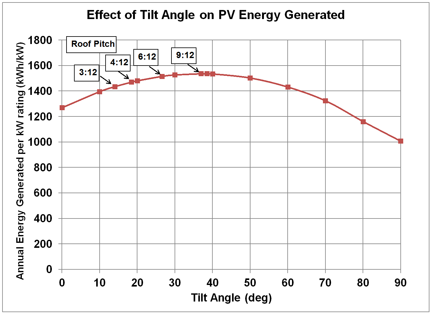

Figure 2.  Effect of Tilt Angle (from Horizontal) on Annual PV Energy Generated per kW DC Power Rating for PV System, at Azimuth Angle of 169 Deg. (11 E of S).

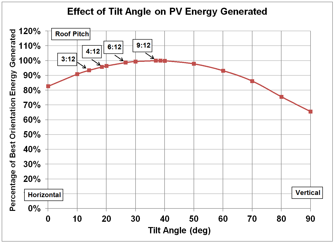
Figure 3.  Effect of Tilt Angle (from Horizontal) on Annual PV Energy Generated as a Percentage of the Energy Generated at the Optimum Tilt Angle, at Azimuth Angle of 169 Deg. (11 E of S).

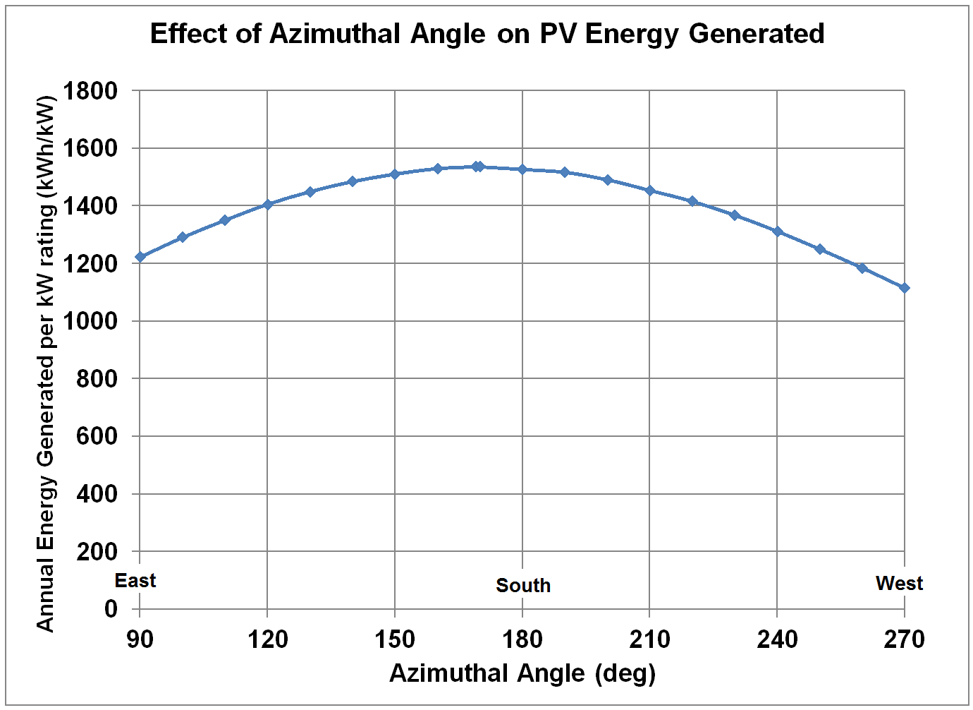
Similarly, the effect of changing the azimuthal angle (rotating the panels around a vertical axis) to point the panels from due east to due west, while fixing the tilt at the optimum 38.5˚ is shown in Figures 4 and 5.  Figure 4 shows the PVWatts Version 2 predictions for annual energy collected per kW DC rating for various azimuth angles.  Interestingly, the predicted energy does not peak at due south, but rather at 11˚ east of due south.  This result for optimum orientation is due to two effects.  First, the air temperatures are lower in the morning, when the sun is in the eastern sky, than in the afternoon, when the sun is in the western sky, especially in this high mountain desert.  Since PV panel output decreases with increasing panel temperature, an eastern orientation would be favored.  Secondly, the summer weather pattern in this Rocky Mountain Valley is for clear weather in the morning, with clouds in the mid and late afternoon, so again, an eastern orientation would be favored.   

Figure 5 shows the same information as Figure 4, but expressed as the annual energy generated at different azimuthal angles as a percentage of the annual energy generated at the optimum angle of 169˚, all at a tilt angle of 38.5˚.  Note that the predicted energy is at least 90% of the energy at the optimum angle for azimuthal angles ranging from 120˚ (east-southeast) to 225˚ (southwest).  Thus, high PV output is predicted over a wide range of orientations other than due south with tilt set to the latitude.  Therefore, it is not necessary to wait until a house is obtained with optimum roof orientation before installing a PV system, or building a complicated rack mounting system to orient the panels differently than the roof. 

Figure 4.  Effect of Azimuthal Angle (due S = 180˚) on Annual PV Energy Generated per kW DC Power Rating for PV System, at fixed Tilt of 38.5˚.

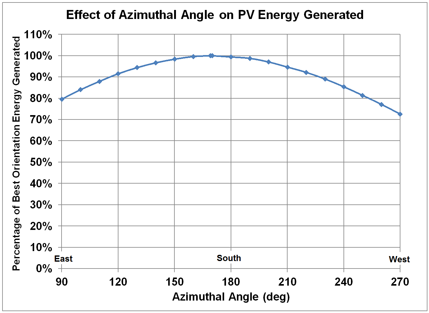
Figure 5.  Effect of Azimuthal Angle (due S = 180˚) on Annual PV Energy Generated as a Percentage of Energy Generated at Optimum Azimuthal Angle, at fixed Tilt of 38.5˚.

It might be unreasonable to compare the normalized output from each system directly, since systems #1 and #2 are at a more favorable orientation than system #3.  For that reason, the output energy from each system is first normalized by the rated power, and then compared with the computer model PVWatts Version 2 (40-km grid) that accounts for the orientation of the panels as well as geographic location (same for all three systems) to predict output energy for PV systems.  By examining the measured energy output of the PV systems and comparing it with the predicted output from PVWatts, the different PV panel orientations can be approximately accounted for. 

The other factor that must be included in predicting performance of PV systems is aging of the solid-state solar cells in the PV collectors.  These three systems all use silicon crystals, and the aging of monocrystalline and polycrystalline silicon solar cells has been studied.  A summary of field degradation studies has been presented by Vazquez and Rey-Stolle (2008), and they conclude that the yearly linear degradation must be less than 0.5% if the panels are to meet the 25-year warranty of at least 80% of the rated power at that time.  Based on their literature survey and others, a linear degradation factor of 0.65% per year has been selected for the results presented here.  Therefore, the PVWatts predicted energies and the projected field energy measurements have been adjusted to reflect the 0.65% per year degradation factor. 

How can the aging factor be accounted for when using the PVWatts computer model?  The aging factor is one of a number of factors that is included in the “derate” factors that are used to adjust between the rated DC power at standard test conditions and the expected power when operating in the field.  The standard aging factor is 1.0 (new array) as shown in Table 2, but this can be adjusted downward as appropriate.  Also shown in Table 2 are the derate factors recommended by NREL for use in PVWatts, as well as factors recommended by SunPower for their systems.  For this work, the overall derate factor of 0.770 as recommended by NREL was used for the first year of operation, and then this factor was reduced by 0.65% for each year beyond the first year. 

Table 2.  Derate Factors for Use in PVWatts Computer Model, showing both the Default Values Recommended by NREL and those Recommended by SunPower for their Systems. 

References for the derate table above:
1 – Photon Magazine article on LID
2 – Show table with up-to-date module flash test average and distribution for modules most often sold into RLCC
3 – Include spec sheets for inverters most often used in RLCC, or show table with CEC efficiency values for these inverters and reference CEC website link.
4 – show representative electrical schematic of SunPower system, including take-offs to show wire lengths and gauges. Show simple calculation of ohmic losses in DC side based on average annual array current from PVSim. Also show placement of inverter relative to breaker, and show similar ohmic loss calculation for AC side.
5 – reference SunPower soiling papers from IEEE 2006 and PVSEC 2007

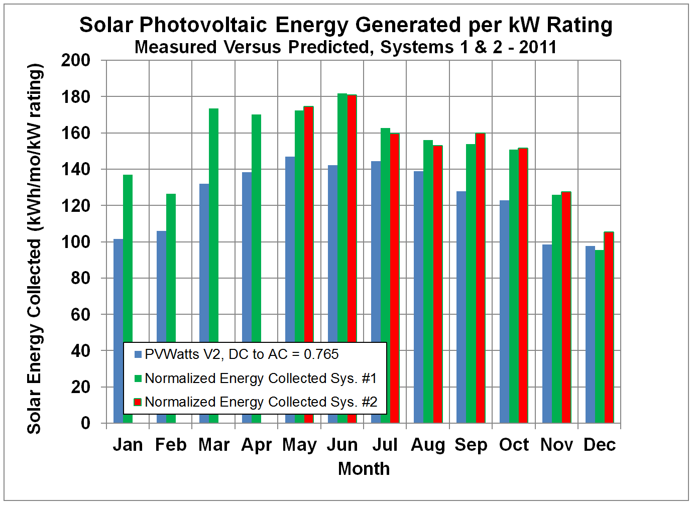
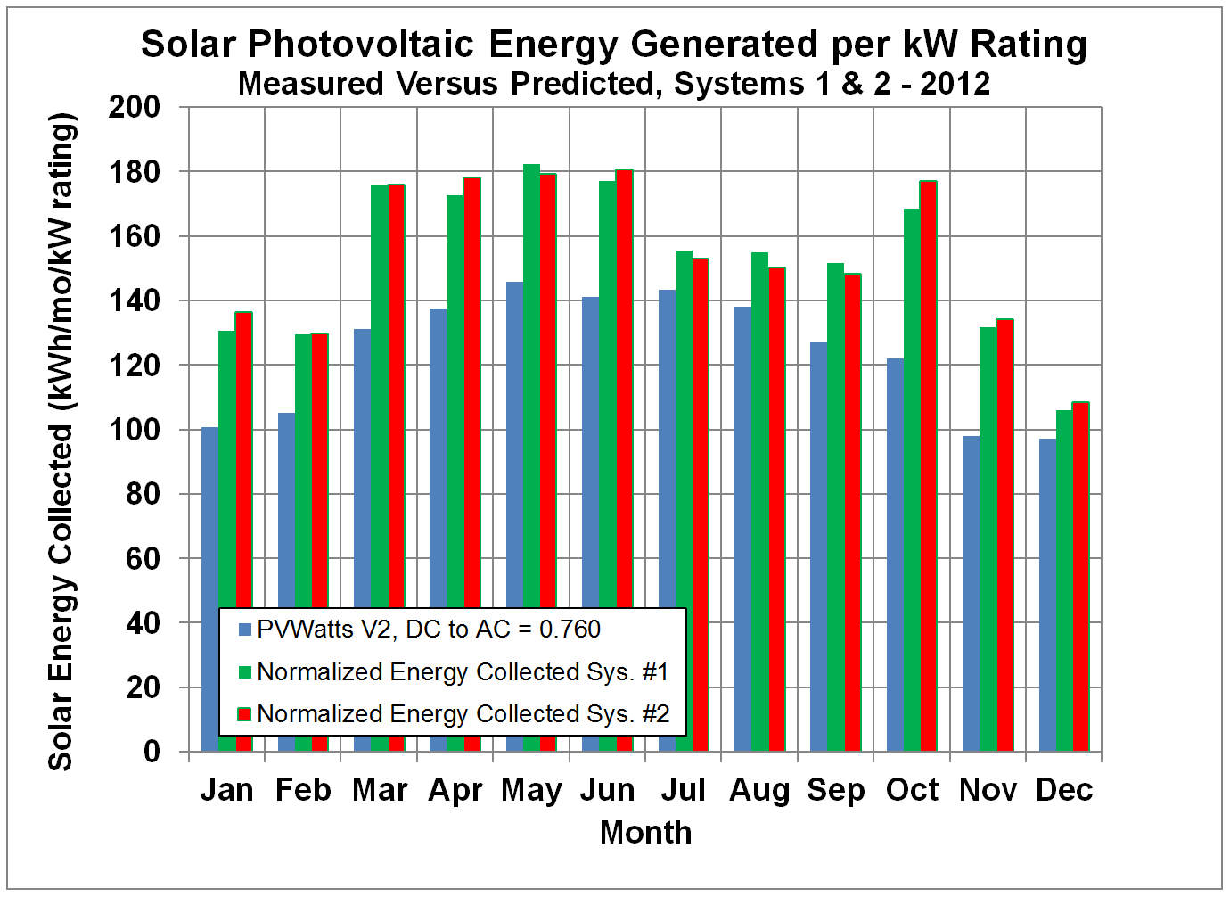
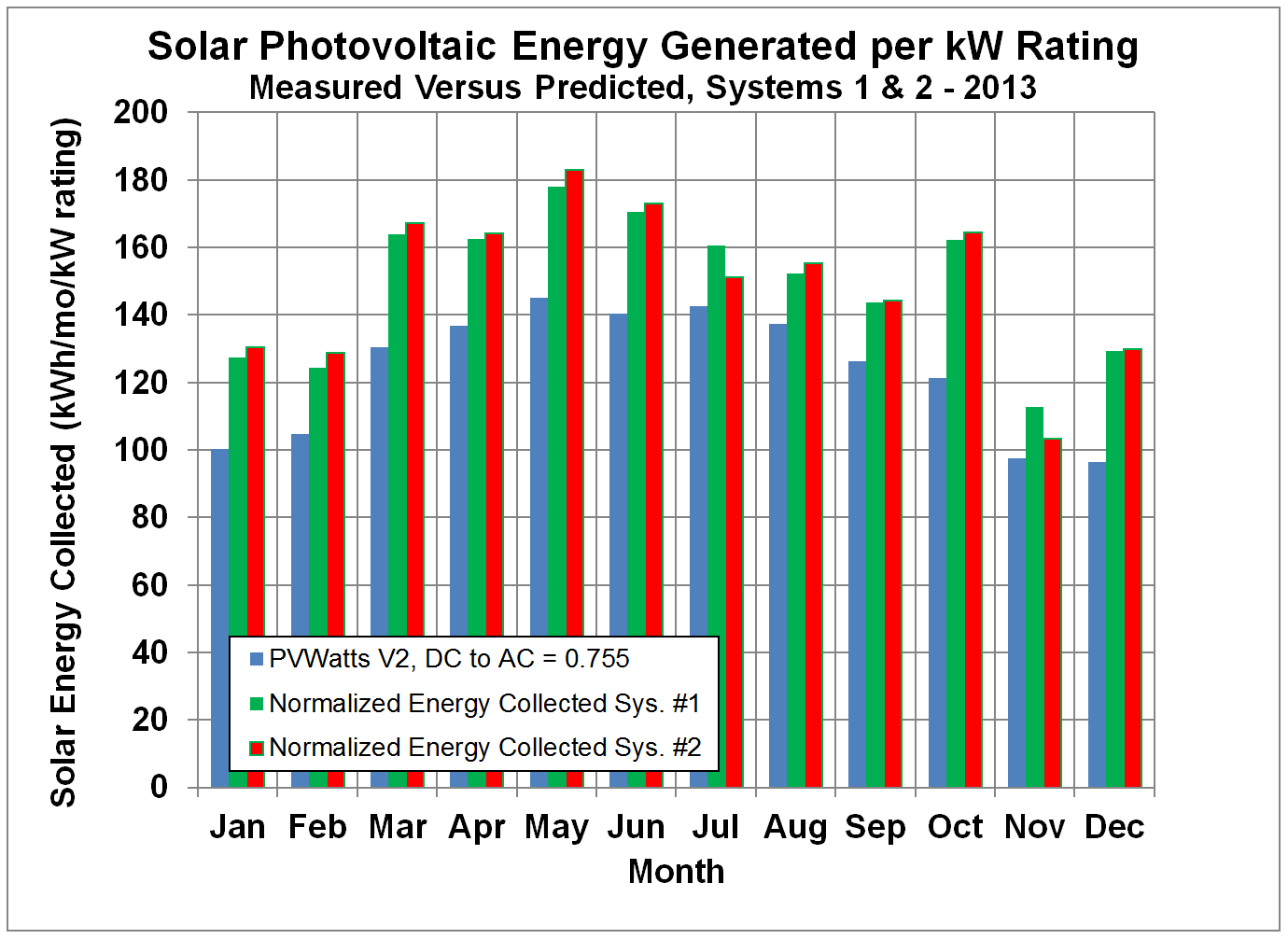
Figure 6 shows the measured monthly energy collected divided by the rated DC power for PV systems #1 and #2 for 2011, Figure 7 shows the data for 2012, Figure 8 shows the data for 2013, and Figure 9 shows the data for 2014.  These systems are made by different manufacturers and have very different efficiencies, but the measured monthly energies normalized by the power ratings are essentially identical within the scatter of the data.  The energy collected by both systems exceeded the predictions by PVWatts.  Over the first year of operation, system #1 exceeded the PVWatt’s prediction by 23.8%.  Over the following years, the output continues to exceed PVWatt predictions.  

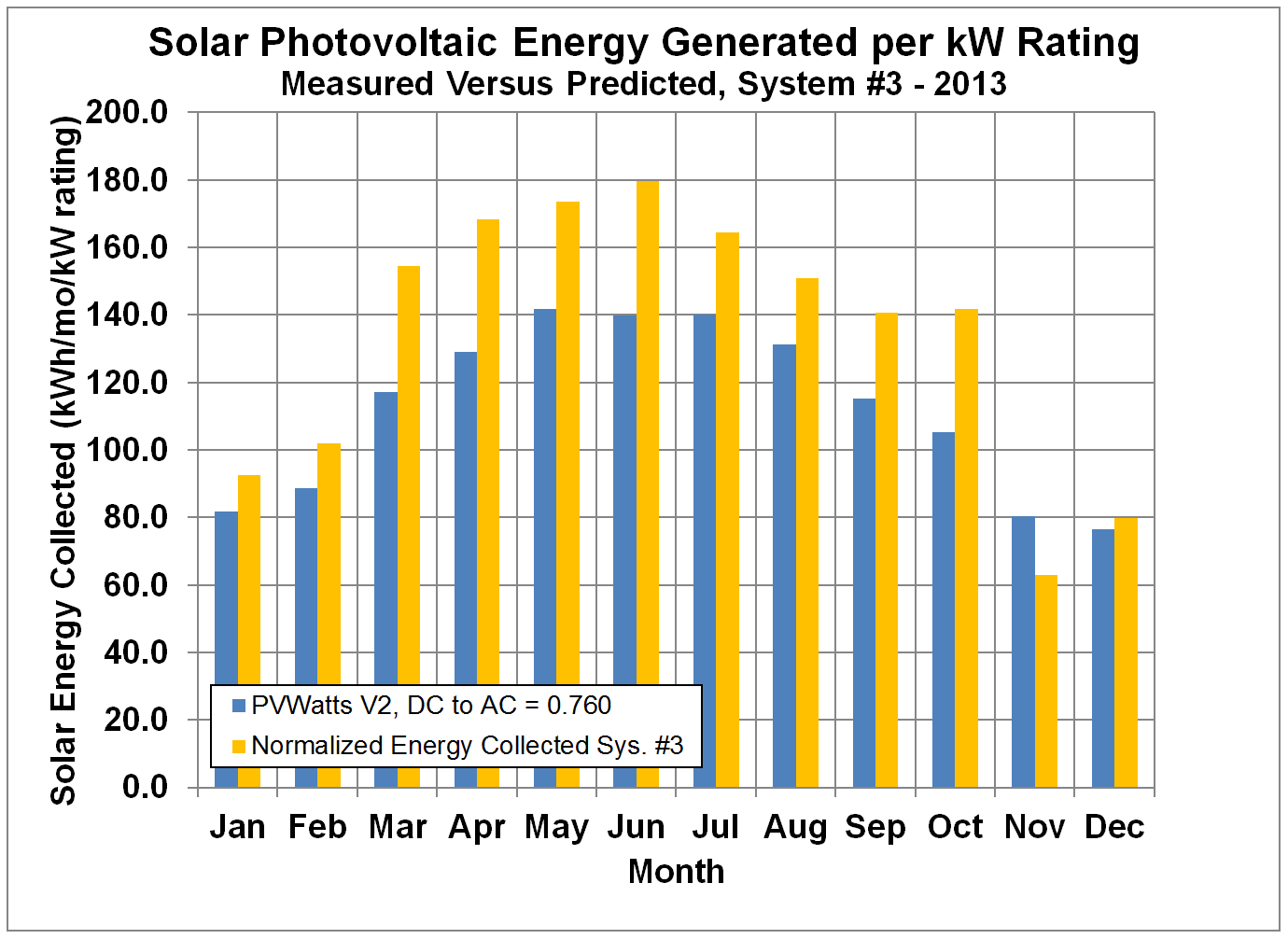
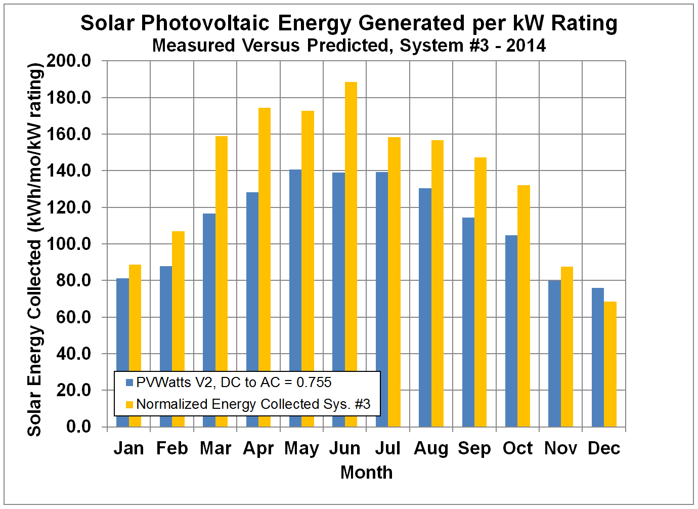
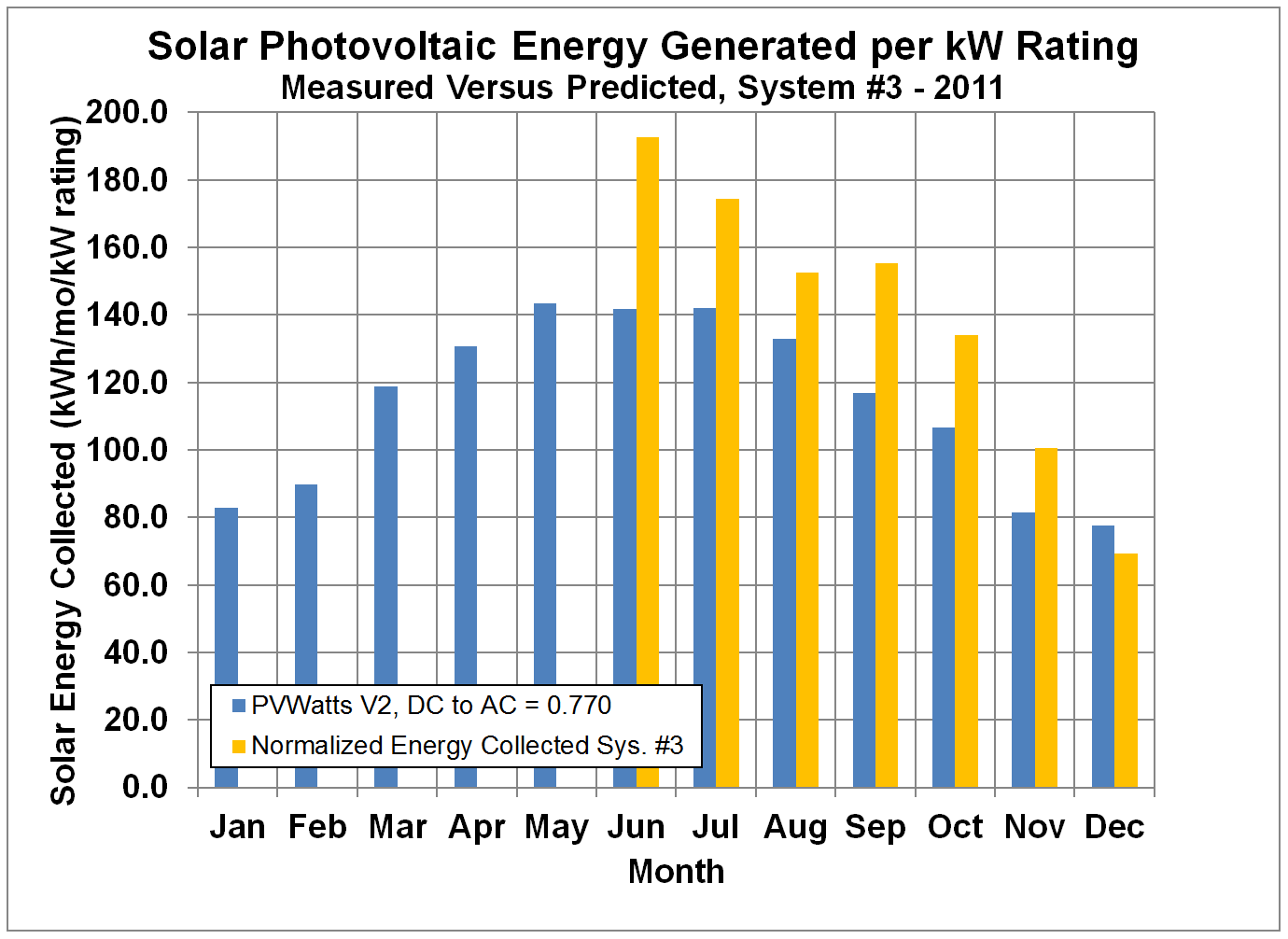
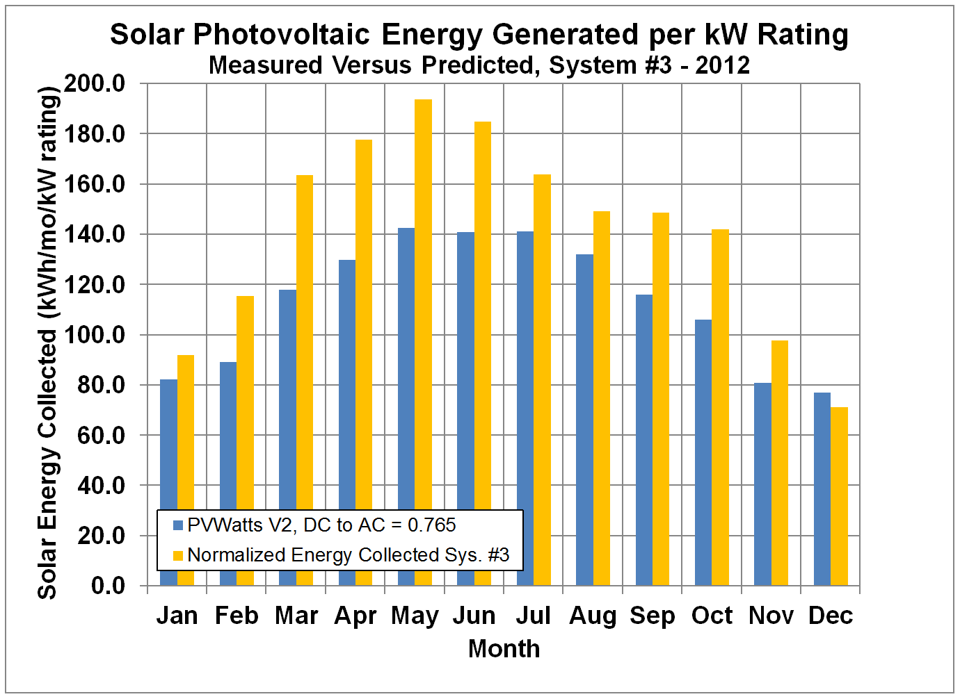
Figure 10 shows the measured monthly energy collected divided by the rated DC power for PV system #3 for 2011, Figure 11 shows the data for 2012, Figure 12 shows the data for 2013, and Figure 13 shows the data for 2014.  System #3 also appears to exceed the PVWatts predictions.  Because of the lower tilt angle for system #3 compared to the other two systems, the predicted power drops off more sharply in the winter compared to the summer.  

Figure 6.  Normalized Monthly Solar Energy Collected by Systems #1 and #2 compared to Predictions by PVWatts with Default DC to AC Conversion Factor, but Adjusted for Age for 2011.

Figure 7.  Normalized Monthly Solar Energy Collected by Systems #1 and #2 compared to Predictions by PVWatts with Default DC to AC Conversion Factor, but Adjusted for Age for 2012.

Figure 8.  Normalized Monthly Solar Energy Collected by Systems #1 and #2 compared to Predictions by PVWatts with Default DC to AC Conversion Factor, but Adjusted for Age for 2013.

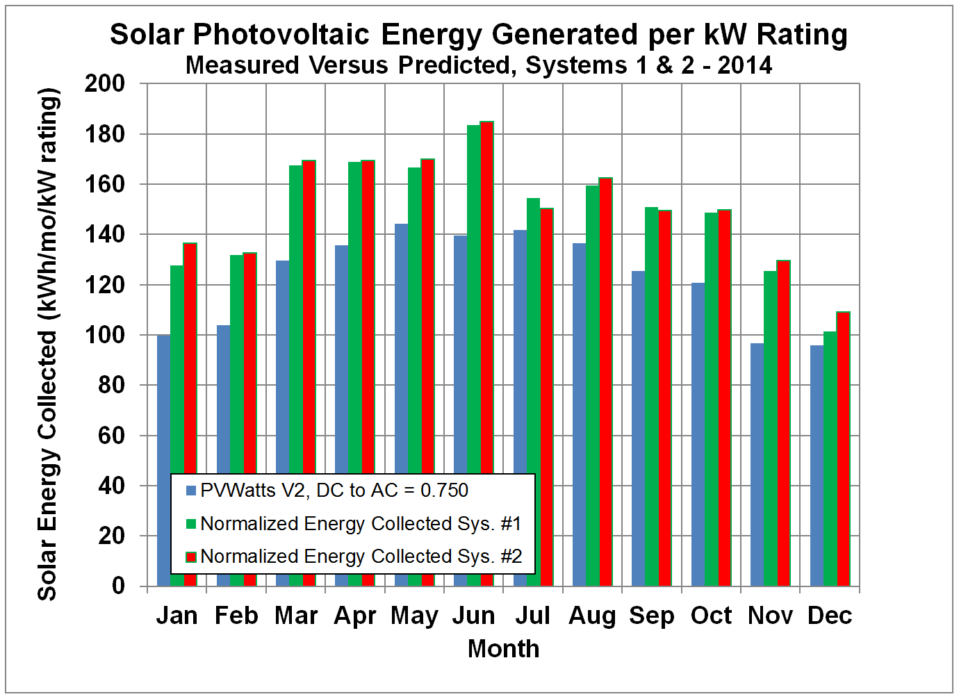
Figure 9.  Normalized Monthly Solar Energy Collected by Systems #1 and #2 compared to Predictions by PVWatts with Default DC to AC Conversion Factor, but Adjusted for Age for 2014.

Figure 10.  Normalized Monthly Solar Energy Collected by System #3 compared to Predictions by PVWatts with Default DC to AC Conversion Factor for 2011.

Figure 11.  Normalized Monthly Solar Energy Collected by System #3 compared to Predictions by PVWatts with Default DC to AC Conversion Factor for 2012.

Figure 12.  Normalized Monthly Solar Energy Collected by System #3 compared to Predictions by PVWatts with Default DC to AC Conversion Factor for 2013.

Figure 13.  Normalized Monthly Solar Energy Collected by System #3 compared to Predictions by PVWatts with Default DC to AC Conversion Factor for 2014.

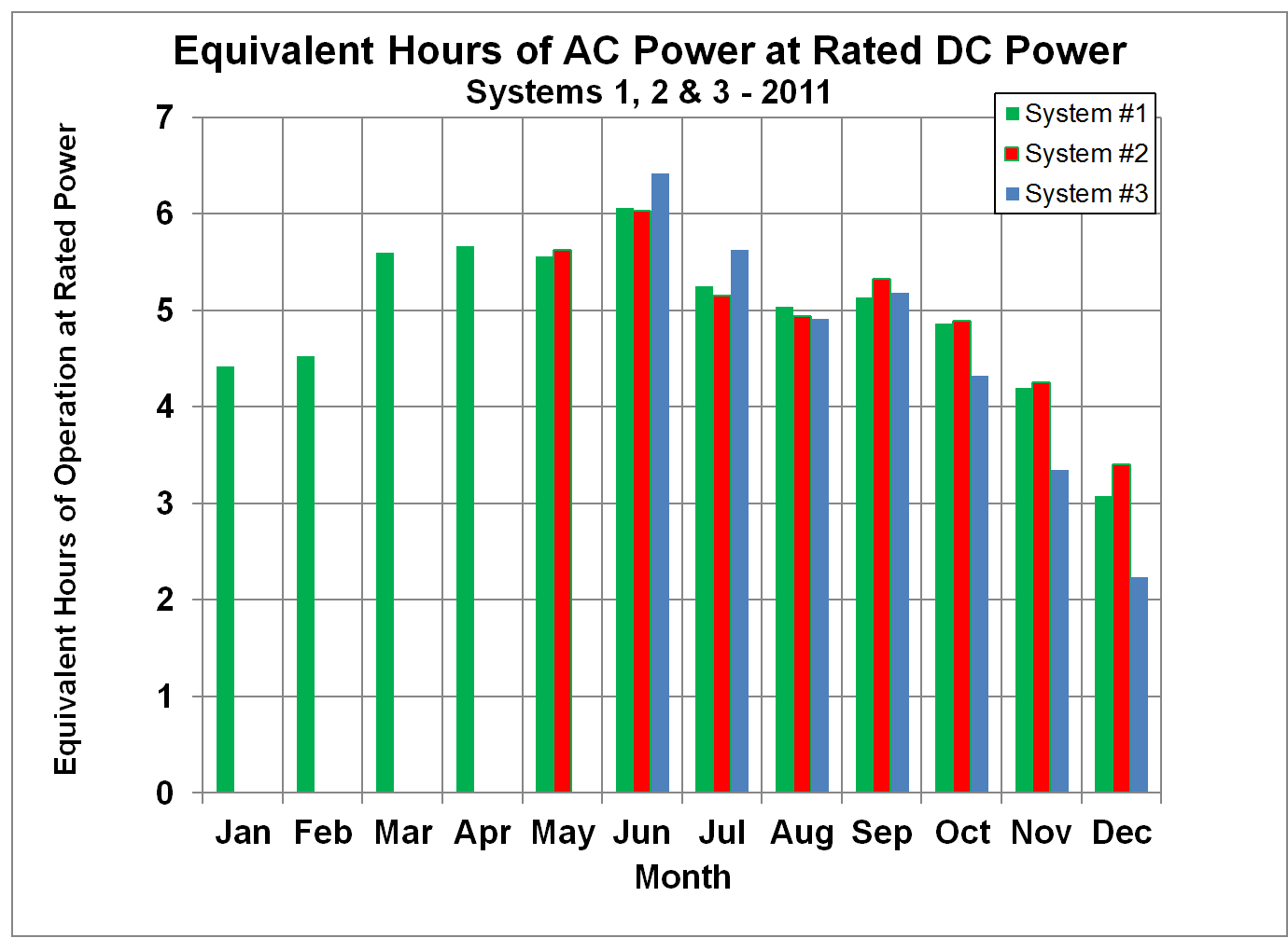
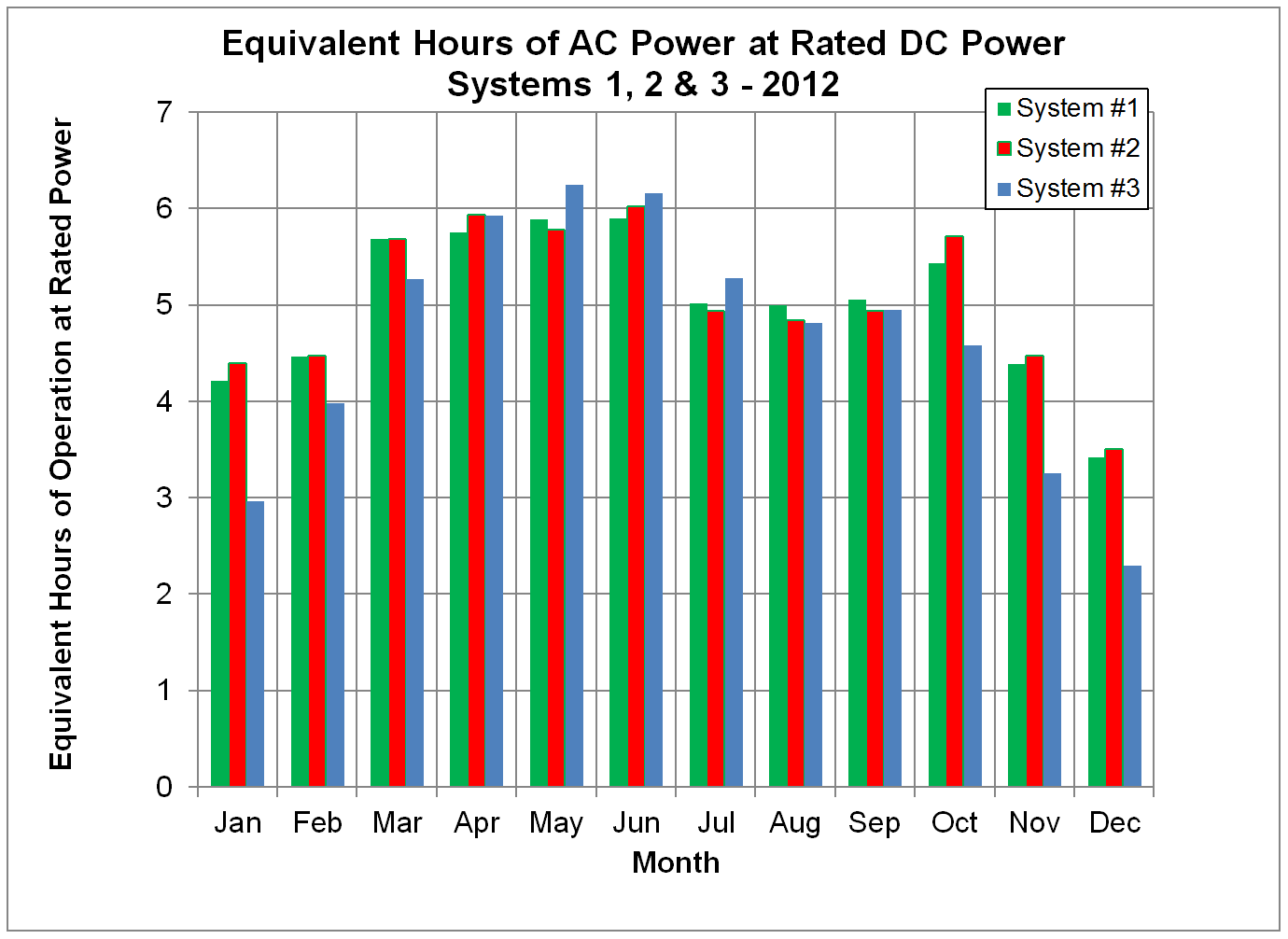
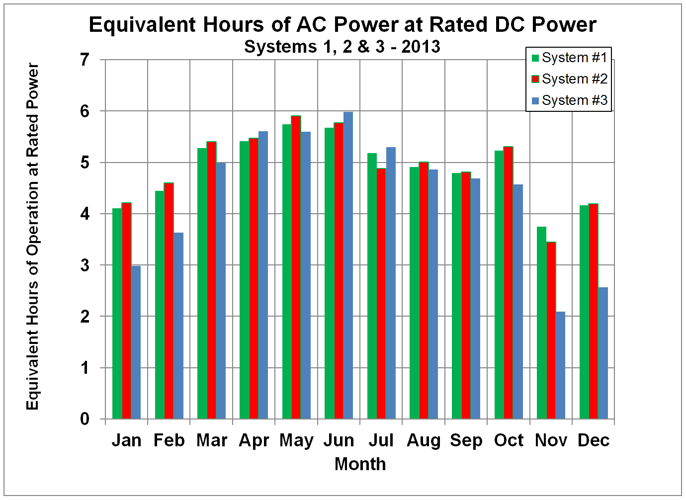
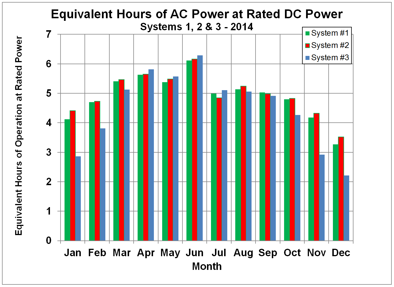
Another way to compare the performance of different solar PV systems is to take the measured energy outputs from the systems that are shown in Figures 6 through 13, which have units of (kWh/mo)/kW rating and divide by the days per month.  This results in overall units of hr/day, and can be interpreted as equivalent hours per day that the system is producing AC power at the full DC rated power.  Such a comparison is shown in Figures 14-17, which show systems #1 and #2 to be performing about the same, just as in Figures 6 - 9, with system #3 producing more energy in the summer months and less in the winter, as expected from its lower tilt angle. 

Figure 14.  Comparison of Normalized Output Energy from Three Solar PV Systems expressed as Equivalent Hours of AC Power at the Rated DC Power Rating for 2011. 

Figure 15.  Comparison of Normalized Output Energy from Three Solar PV Systems expressed as Equivalent Hours of AC Power at the Rated DC Power Rating for 2012. 

Figure 16.  Comparison of Normalized Output Energy from Three Solar PV Systems expressed as Equivalent Hours of AC Power at the Rated DC Power Rating for 2013. 

Comparisons between PVWatts Predictions and Measured Energy

For the three systems tested, the actual measured collected energy exceeded the PVWatts V.2 predictions by about 20% or more.  It is not typical that actual energy production is this much in excess of PVWatts’ predictions.  Gostein et al. (2009) collected data from over 480 residential and commercial installations of PV systems in Austin, Texas, USA.  They found that PVWatts (V.1) predicted energy production was about 8% higher than the measured energies of the PV systems.   

Dean (2010) examined the discrepancies for model results and concluded that the main area for discrepancies was not in model algorithms, but rather in the input data for solar radiation.  Because of variability in solar radiation from day-to-day, month-to-month, and year-to-year, some method must be used to select an average dataset or a typical dataset to use as input to the simulation to compute electrical energy generated by the solar PV system.  The radiation data used by NREL in PVWatts comes from the Typical Meteorological Year data set, version 2, abbreviated as TMY2.  This dataset contains hourly values of solar radiation, and is derived from 30 years (1961-1990) of historical data for 230 locations across the USA from the National Solar Radiation Database (NSRDB).  Data for two of the years were removed from the data set due to large volcanic eruptions during those years.  For each month, an algorithm is used to select the “most typical” month of the thirty years in the database. The algorithm minimizes the difference between the year in question and the long-run average for each parameter.  Dean points out some shortcomings of this approach, and questions whether this “typical” dataset used to define TMY2 results in values that are “central,” or mean, or median.

Dean (2010) went back to the original NSRDB dataset that includes the full 30 years worth of data, and processed those results using quantitative risk analysis, which is a statistical approach to process the large dataset.  Further, he developed a reduced form model using a neural network, as a part of this analysis.  For the particular dataset that he chose in Newark, New Jersey, his analysis showed that the PVWatts results using the TMY2 dataset resulted in a 6% higher energy production than his more complete statistical analysis.  Of course, to accept Dean’s results requires faith in the neural network model, which is not physically based, but it will be assumed that it was implemented accurately.  He suggests that for the limited comparisons that he performed, that the TMY2 dataset was biased toward higher solar radiation levels than average levels, and this was the source of the high predictions by PVWatts (V.1).  Dean also points out that Peppers (2006) showed empirical evidence that PVWatts (V.1) over-predicted field measurements by 10%. 

Yates and Hibbert (2010) compare the performance of several simulation codes with measured data for two locations in California.  The PVWatts predictions for the first case were 2.5% lower than the measured energy, while the PVWatts predictions for the second case were 8.5% low relative to measured values.  Enphase Energy in their advertising brochures indicate that solar PV systems with their microinverters provide energy that exceeds PVWatts predictions by an average of 8%. 

Based on the above comparisons, the PVWatts predictions are generally within ±10% of the measured values.  Therefore, it seems odd that the three systems tested in this location appear to produce more than 20% higher energies than the PVWatts predictions.  It is likely the interpolation scheme used to estimate the solar insolation for this local area does not properly account for the high altitude of this location, and the higher solar insolation.  It is likely that users in this immediate area can expect performance significantly better than what is predicted by PVWatts.   

Application of these Results to other Locations

The results shown here provide a guide to estimate PV systems output energy based on the DC power rating.  However, an additional parameter must be considered to interpret these results, and that is the solar insolation (or radiation or irradiation).  The three systems shown here all operate similarly in terms of collected energy per unit kW rating only because they are exposed to the same solar insolation.  To apply these results to other parts of the country or the world, the results must be scaled based on the solar insolation at the point of interest divided by the solar radiation these panels were exposed to, which is a yearly average of about 5.78 kW/m2/day.  See Figure 1 to estimate solar insolation for other parts of the U.S., or use PVWatts V2 for a more precise value (http://mapserve3.nrel.gov/PVWatts_Viewer/index.html).  For the U.S. the results presented here should be roughly typical for the southwestern U.S., while other parts of the country have lower solar insolation), and therefore, lower energy per DC kW rating of the panels. 

Economics for Residential Solar PV Systems in Southern Colorado

The generation of electricity from solar PV panels has generally not been cost competitive with electricity generated by large utility plants in the past.  Two things have changed that have made the solar PV systems more cost competitive.  First, significant subsidies from the federal government and from local utilities have reduced the effective cost to residential customers.  Second, these subsidies in the U.S., and sometimes even more generous subsidies outside the U.S. have resulted in production increases, with the result that production costs and retail prices have been reduced. 

The federal government in the U.S. provides a 30% credit for solar PV systems purchased for residential use.  Utility subsidies are quite variable in both time and place, but can be larger than the subsidies from the federal government.  Some states, mostly in the northeastern U.S. also have solar renewable energy certificates (SREC’s) that provide a market for the credits, providing an additional source of revenue for owners of solar PV systems. 

Of course, the solar industry is not alone is being a subsidized energy source.  There is the Price-Anderson Nuclear Industries Indemnity Act that limits the nuclear industry to pay only the first $12.6 billion in damages from a nuclear accident.  (The costs of the Japanese tsunami-nuclear disaster have dwarfed this figure.)  Also the research performed by the Atomic Energy Commission, which was followed by the Energy Research and Development Administration, which was followed by the Dept. of Energy is paid for predominately or completely from federal taxes. 

The oil industry has its three favorite deductions: (1) domestic manufacturing deduction, (2) a deduction for treating royalties paid to foreign governments as deductible taxes (sort of the opposite of the first deduction), and (3) intangible costs deductions.  This list does not include the cost of foreign wars in oil rich nations, wars that might be regarded as trying to secure future oil supplies.  The war in Iraq has been estimated to have cost about $1,000,000,000 U.S. dollars to date.  Thus, the argument that the economics of solar energy should be computed on a non-subsidized basis would require that the costs for the competing energy sources such as nuclear and oil also be adjusted for subsidies, probably an impossible task.  So the only realistic comparison is for each energy source at the final cost to the consumer.    

In spite of the subsidies for the U.S. oil industry, the production of crude oil in the U.S. has declined dramatically since 1985, as shown in Figure 18.  M. King Hubbert (1956) created and first used models to predict that United States oil production would peak between 1965 and 1970.  The actual peak occurred 15 to 20 years later than his predictions, but just as he predicted, the production has been steadily declining after this peak in production.  Similar models indicate that peak oil production world-wide will occur around the present time (2010).  This decline in crude oil production emphasizes the need to find renewable energy sources, and provides a motivation for studying solar energies such as PV systems for electrical generation. 

The costs to the homeowners for the PV systems are known, but maintenance costs are unknown.  From examining the literature and discussions with a solar PV installer, it is assumed that the inverters for the PV systems will last 12 to 15 years, so that the inverters will require replacement once over 25 years.  The cost for a SunPower 3000m inverter is about $2312, and a labor cost of $500 has been estimated for replacement.  Additional maintenance over 25 years has been estimated at $500.  All of these costs are listed in Table 3, and they can be summed to estimate a total cost for 25 years of operation, with the further assumption that the system is obsolete after 25 years.  If the energy output for these systems can be estimated for the same period, then the cost per unit electrical energy can be computed and compared with commercial rates.

Figure 18.  Production of Oil in the United States. 

The energy output from system #1 has been monitored for over a year.  The energy output for system #2 has been monitored for a shorter time, but it seems to produce the same energy per kW rating as system #1 as shown in Figures 6 - 9.  The output from system #3 relative to the PVWatt’s model predictions is similar to systems #1 and #2, as shown in Figures 10 - 13.  Therefore, the annual performance of system #1 can be used to estimate the output of system #2 by just scaling based on the rated system power.  The performance of system #3 can be estimated as the annual output from system #1 scaled by the predicted annual energy from PVWatts for the two systems including the effect of the different power ratings.  These estimated annual energy outputs have been extrapolated to 25 years worth of performance, with each year linearly decreased from the previous year by 0.65%, the annual degradation factor discussed above, with results presented in Table 3. 

Since both the PV system costs and output energies have been estimated as shown in Table 3, the cost per kWh can be computed.  Those results are shown in Table 3 as “Cost per solar kWh over 25 years.”  Those results are compared with the electricity costs when purchased from the appropriate utilities, and these results are shown in Table 3.  The cost from utilities is different for system #3 than for #1 and #2 since a different utility serves the respective areas.  In this part of southern Colorado, a homeowner can only choose the one utility that offers service in the area.

Table 3.  Initial Costs, Estimated Maintenance Costs, Estimated Performance, and Energy Costs for the Three Solar PV systems.

As can be seen in Table 3, the cost for the solar PV generated electricity amortized over 25 years is less than the current cost of electricity from the utilities.  However, most people do not live in their homes for 25 years.  Thus, to recoup the initial investment, the value of the home would have to reflect the value of the solar PV system.  A report by Hoen, et al. (2001) reports that homes in California with solar PV systems sold at a premium of about $5.50/watt (approximately the unsubsidized cost of a PV system) compared to comparable homes with PV systems, or roughly the cost of a new PV system.  Most of the surveyed homes had relatively new PV systems with a typical size of 3.1 kW, and the price premium tended to decrease for older PV systems, as would make sense.  Since the PV market is larger in California than in any other states, caution must be used in extrapolating these results to other states.  However, it is reasonable to expect that as solar PV systems become more widespread, this same increase in resale home value with PV systems might be expected.

Another way to look at cost analysis of PV systems is to compute the payback period, that is, how many years will it take to pay back the initial investment.  If a simple payback calculation is performed, it ignores the potential increase in energy prices, as well as the cost of money for the initial investment.  (These assumptions are explored below.)  In this analysis, the projected decrease in PV system output of 0.65% per year is included.  The simple payback for system #1 is 9 years, for system #2 is 12 years, and for system #3 is 11 years.  After this payback time, the systems provide “free” electricity for the balance of the 25-year lifetime, except that a first inverter replacement would be a likely additional cost at 12 to 15 years after installation.  The panels are guaranteed to still produce 80% of rated power at 25 years, so the actual lifetime is expected to be longer than 25 years, but a second inverter replacement would need factored in for longer lifetime projections.

The simple cost analysis shown in Table 3 does not include the likely inflation rate for electricity costs, nor the cost of money used to invest in the PV systems.  Some comments can be made concerning these factors.  Estimating inflation rates into the future is difficult given the background of the very high inflation rates during World War I and II and of the 1970’s contrasted with the low inflation rates of the 1930’s, the 1950’s, and more recent years.  The average retail price of electricity to residential customers over the period 1997 to 2009 is shown in Figure 19, and the average inflation rate as computed using a least-squares error fitting procedure is computed to be 3.07%.  Much of the new generating capacity uses natural gas as the fuel of choice, and the average retail price of natural gas to residential customers is shown in Figure 20 for the period 1989 through 2010.  Using a least-squares error fitting procedure, the natural gas inflation rate over this period was 4.69%.  A cap-and-trade policy to reflect the cost of build-up of greenhouse gases in the atmosphere might cause the energy inflation rate to increase at a faster rate than the past historical rate. 

How do these inflation rates for energy compare to overall inflation rates for all commodities?  The consumer price index from 1913 through 2010 is shown in Figure 21.  It is clear that over that period, inflation rates have varied dramatically, with higher inflation rates during major wars and the energy crisis of the 1970’s, and lower rates during recessions and depressions.  The average inflation rate over the extended period from 1913 through 2010 was computed to be 3.58% using a normalized least-squares error fitting.  However, the inflation rate over the more recent periods corresponding to the data shown for electricity in Figure 19 and natural gas shown in Figure 20 are lower.  For the period 1997 through 2009, the CPI inflation rate was 2.68% compared to the inflation rate for electricity of 3.08%.  For the period 1989 through 2010 the CPI inflation rate was 2.64% compared to the inflation rate for natural gas of 4.69%. 

The conclusion is that energy prices appear to have an inflation rate similar to, but higher than, (much higher for natural gas) the overall inflation rate as measured by the CPI.  It is possible that with “peak oil” already having occurred, and with high growth economies in Asia and South America, that future energy prices will escalate at a faster rate that what has occurred over the last decade or two, but this is only speculation at this point.

Currently long term investments in bank accounts draw about 1% or less, while long-term mortgages are at about 3.5%.  Therefore, the cost of money is similar to the overall inflation rate, and also similar to, or lower than, the inflation rate for energy.  Thus, the simple analysis above using fixed 2011 U.S. dollars is a reasonable first step for estimating return of solar PV systems, although the actual return might be better than shown if the cost of energy continues to inflate at rates higher than the overall cost of living.

It should be noted that solar PV systems my now be leased in many parts of the U.S. and perhaps in the rest of the world.  In some cases, the lease agreements require no up-front cost by the homeowner, but only a monthly payment.  Analysis of these lease agreements is outside the scope of this report, but might be an attractive option for homeowners wanting to avoid the large up-front investment.    

The economic analysis presented here is influenced by the following factors: initial system cost, solar insolation (5.78 kW/m2/day in this area), utility rates, and rebate amounts by governments and utilities.  So these factors should be taken into account in using these results to apply to other parts of the world.

Figure 19.  Average Retail Price of Electricity to Residential Customers in the United States over the Period 1997 – 2009.

Figure 20.  Average Cost of Natural Gas to Residential Customers in Colorado over the period 1989 – 2010.

Figure 21.  The Consumer Price Index over the Period 1913 thorough 2010, and Inflation Rates Calculated for Various Time Periods. 

References:

Dean, S.R. (2010).  “Quantifying the Variability of Solar PV Production Forecasts,” SOLAR 2010 Conference Proceedings. 

Gostein, M., Hershey, R., Dunn, L., Stueve, B. (2009).  “Performance Analysis of Photovoltaic Installations in a Solar America City,” Photovoltaic Specialists Conference (PVSC), 2009 34th IEEE.

Hoen, B., Wiser, R., Cappers, P., and Thayer, M. (2011).  “An Analysis of the Effects of Residential Photovoltaic Energy Systems on Home Sales Prices in California,“ Lawrence Berkeley National Laboratory report LBNL-4476E. Download from http://eetd.lbl.gov/ea/emp/reports/lbnl-4476e.pdf.    

Hubbert, M. K. (1956). "Nuclear Energy and the Fossil Fuels 'Drilling and Production Practice'". Spring Meeting of the Southern District. Division of Production. American Petroleum Institute. San Antonio, Texas: Shell Development Company. pp. 22–27. http://www.hubbertpeak.com/hubbert/1956/1956.pdf.

Marion, B., Anderberg, M., George, R., Gray-Hann, P., and Heimiller, D. (2001).  “PVWATTS Version 2 – Enhanced Spatial Resolution for Calculating Grid-Connected PV Performance,” NREL Report NREL/CP-560-30941, presented at the NPCV Program Review Meeting. 

Pepper, J. (2006).  Comments of Clean Power Markets, Inc. on CPUC Energy Division Staff Draft Proposal Phase I for the California Solar Initiative Design and Administration 2007-2016, Filed under Rulemaking 06-03-004, CPUC, May 16, 2006

Vazquez, M., and Rey-Stolle, I. (2008).  “Photovoltaic Module Reliability Model Based on Field Degradation Studies,” Prog. Photovolt: Res. Appl. Vol. 16: 419-433. 

Yates, T., and Hibbert, B. (2010).  “Production Modeling for Grid-Tied PV Systems,” Solar Pro,  pp. 30-56, April/May, 2010.